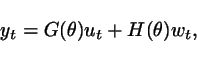
- LSCR is a general method for system identification.
- differently from standard identification methods, LSCR does not deliver a single model; instead, it delivers a model set.
- as the amount of information increases, the model set shrinks around the true system and - for any finite sample size - the set contains the true system with a guaranteed probability chosen by the user.
The need for a set of models
Even when a system  belongs to the model class, we cannot expect that a model
  identified
from a finite number of data
coincides with since there are a number of noise
sources affecting our data: measurement noise,
presence of disturbances acting on the system, etc.
identified
from a finite number of data
coincides with since there are a number of noise
sources affecting our data: measurement noise,
presence of disturbances acting on the system, etc.
As a consequence, under general
circumstances the only
probabilistic claim we are in a position to make is that
which
is clearly
a useless statement if our
intention is to credit the model with reliability.
To obtain certified reliability
results, one can move from nominal-model to model-set identification.
The
situation is depicted in Figure 1:
for any number of data points N, the parameter estimate is affected
by random fluctuation, so that it has probability zero to exactly hit
the true system parameter value ![]() . Considering a region around the
estimate,
however, elevates the probability that
. Considering a region around the
estimate,
however, elevates the probability that ![]() belongs to the region
to a nonzero - and therefore meaningful - value.
belongs to the region
to a nonzero - and therefore meaningful - value.
![\includegraphics[width=5.5cm]{region-around-estimate.eps}](equations-figures/img24.png)
This observation points to a
simple, but important fact:
Challenging the
reader with a
preliminary
example
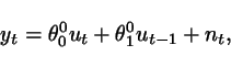
Consider the system
Assume
we know that ![]() is an
independent process with symmetric distribution around
zero. Apart from this, no knowledge on
is an
independent process with symmetric distribution around
zero. Apart from this, no knowledge on ![]() is assumed: it can
have any (unknown) distribution: Gaussian; uniform; etc. Its variance
can be any (unknown) number, from very
small to very large. We do not even make any stationarity assumption on
is assumed: it can
have any (unknown) distribution: Gaussian; uniform; etc. Its variance
can be any (unknown) number, from very
small to very large. We do not even make any stationarity assumption on
![]() and allow its distribution to vary
with time.
and allow its distribution to vary
with time.
The assumption
that ![]() is independent can be interpreted by
saying that we know the
system structure: it is an autoregressive system of order 1.
is independent can be interpreted by
saying that we know the
system structure: it is an autoregressive system of order 1.
9 data points were generated
according to the system and they are shown in Figure
2.
Can you guess the value of ![]() or give a
confidence region for it?
or give a
confidence region for it?
![\includegraphics[width=7cm]{preview-y-data.eps}](equations-figures/img54.png)
To form a guaranteed confidence region
for ![]() , we use
LSCR.
, we use
LSCR.
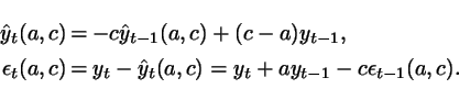
Rewrite
the system as a model with
generic parameter ![]() :
:
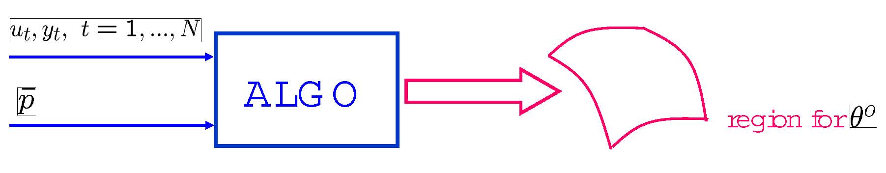
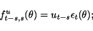
The predictor and prediction error
associated with the model are
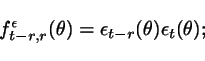
Next
we compute the prediction
errors ![]() for
for ![]() ,
and calculate
,
and calculate
Note
that, ![]() are
functions of
are
functions of ![]() that can indeed be computed from the
available
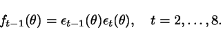
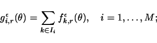
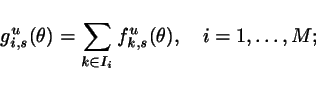
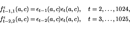
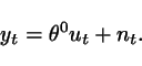
data set. Then, we take different averages of these functions.
Precisely, we form 8 averages of the form:
that can indeed be computed from the
available
data set. Then, we take different averages of these functions.
Precisely, we form 8 averages of the form:
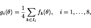
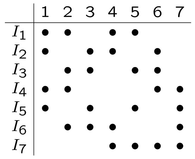
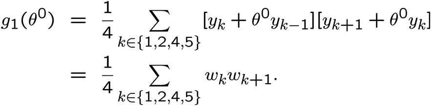
where the sets ![]() are subsets
of
are subsets
of ![]() containing the
elements highlighted by a bullet in
the table below. For instance:
containing the
elements highlighted by a bullet in
the table below. For instance: ![]() ,
, ![]() ,
etc. The functions
,
etc. The functions ![]() ,
, ![]() ,
can be interpreted as
empirical 1-step correlations
of the prediction error.
,
can be interpreted as
empirical 1-step correlations
of the prediction error.
Functions ![]() ,
, ![]() ,
obtained for the data in
Figure 2 are
displayed in Figure 3.
,
obtained for the data in
Figure 2 are
displayed in Figure 3.
![\includegraphics[width=7cm]{preview-correlations.eps}](equations-figures/img72.png)
Fig.3 The ![]() functions.
functions.
Can you now guess the value of ![]() ?
?
Let me give you a hint: the ![]() functions have a tendency to
intersect the
functions have a tendency to
intersect the ![]() -axis near
-axis near ![]() . Why is it so?
Let us
re-write one of these functions, say
. Why is it so?
Let us
re-write one of these functions, say ![]() ,
for
,
for ![]() as follows:
as follows:
The right-hand-side is zero mean and, due
to averaging, the "vertical displacement" from the zero line
is
reduced. So, we
would like to claim
that ![]() will be "somewhere" near where the
average functions
intersect the
will be "somewhere" near where the
average functions
intersect the ![]() -axis.
-axis.
While the above reasoning makes
sense, LSCR provides us with a much stronger claim:
 is 0.5.
Comments.
1.
The interval is stochastic because
it depends on data; the true parameter value ![]() is not and it
has a fixed location that does not depend on any random element. Thus,
what the above RESULT says is that the interval is random and contains
the true parameter value
is not and it
has a fixed location that does not depend on any random element. Thus,
what the above RESULT says is that the interval is random and contains
the true parameter value ![]() in 50% of
the cases.
in 50% of
the cases.
![\includegraphics[width=3.5cm]{preview-more-trials.eps}](equations-figures/img92.png)
Fig.4 10 more trials.
To better understand the nature of
the result, we performed 10 more simulation trials obtaining the
results in Figure 4. Note that ![]() and
and ![]() were as follows:
were as follows: ![]() = 0.2,
= 0.2, ![]() independent with uniform
distribution between -1 and +1.
independent with uniform
distribution between -1 and +1.
2.
In this example, the probability is
low (50%) and the interval is rather large. With more data, we
obtain smaller intervals and higher probabilities.
3. The LSCR algorithm was
applied
with no knowledge about the noise level or distribution and, yet, it
returned an interval whose probability was exact, not an upper bound.
The key is that the above RESULT is a "pivotal" result as
the probability remains the same no matter what the noise
characteristics are.
4. LSCR works along a
totally different inference principle from standard Prediction Error
Minimization (PEM) methods. In particular - differently from the
asymptotic theory of PEM - LSCR does not construct the confidence
region by quantifying the variability in the estimate.
LSCR for general linear systems
Data generating system
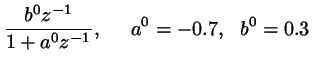
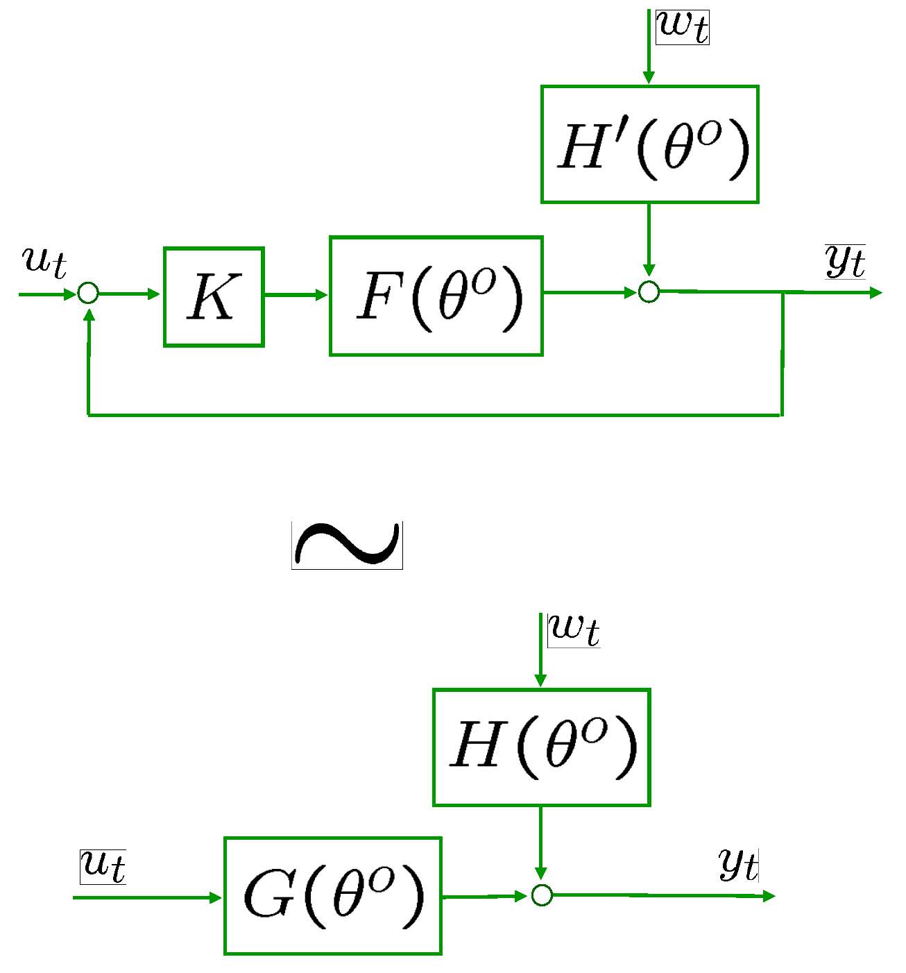
Consider the general linear
system in Figure 5.
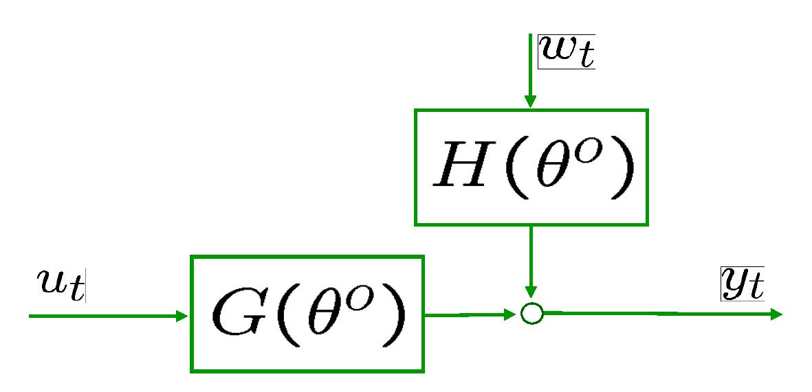
Assume that ![]() and
and ![]() are
independent processes (open-loop). For closed-loop click here.
are
independent processes (open-loop). For closed-loop click here.
No
a-priori knowledge about the noise is assumed.
The basic assumption is
that the system structure is known. Correspondingly, we take a
full-order model class of the form:
Construction of confidence regions
Two types of confidence sets are
constructed: ![]() ,
, ![]() .
.
A confidence regions ![]() for
for ![]() is usually
obtained by taking the intersection of a few of
these
is usually
obtained by taking the intersection of a few of
these ![]() and
and ![]() (see below).
(see below).
------------------------------------------------------------------------------
Procedure for the
construction of ![]()
------------------------------------------------------------------------------
(this generalizes
the preliminary
example)
(1) Compute the prediction errors
for a
finite number of values of ![]() , say
, say ![]() ;
;
(2) Select an
integer ![]() . For
. For ![]() , compute
, compute
(3) Let ![]() and consider a
collection
and consider a
collection ![]() of subsets
of subsets ![]() ,
, ![]() , forming a group
under the symmetric difference
operation (i.e.
, forming a group
under the symmetric difference
operation (i.e. ![]() , if
, if ![]() ). Compute
). Compute
(4) Select an
integer ![]() in the interval
in the interval ![]() and find the
region
and find the
region ![]() such that at
least
such that at
least ![]() of the
of the ![]() functions are
bigger than zero and at
least q are smaller than zero.
functions are
bigger than zero and at
least q are smaller than zero.
Theorem 1 below states that the
probability that![]() is
exactly equal to 1-2q/M. Thus, q is a free parameter the user
can employ to determine the probability of the confidence region.
is
exactly equal to 1-2q/M. Thus, q is a free parameter the user
can employ to determine the probability of the confidence region.
In the procedure for construction
of ![]() , the empirical
auto-correlations in point (2) are
replaced by empirical cross-correlations between the input signal and
the prediction error.
, the empirical
auto-correlations in point (2) are
replaced by empirical cross-correlations between the input signal and
the prediction error.
---------------------------------------------------------------
Procedure
for the
construction of
![]()
---------------------------------------------------------------
(1) Compute the prediction
errors
for a
finite number of values of ![]() , say
, say ![]() ;
;
(2) Select an
integer ![]() . For
. For ![]() , compute
, compute
(3) Let ![]() and
consider a collection
and
consider a collection ![]() of subsets
of subsets ![]() ,
, ![]() ,
forming a group under the symmetric difference operation. Compute
,
forming a group under the symmetric difference operation. Compute
(4) Select an
integer ![]() in the interval
in the interval ![]() and find the
region
and find the
region ![]() such that at
least
such that at
least ![]() of the
of the![]() functions are
bigger than zero and at least
functions are
bigger than zero and at least ![]() are smaller than
zero.
are smaller than
zero.
Comments
1.
The procedures return regions of
guaranteed probability despite that no a-priori knowledge about the
noise
is assumed: the noise enters the procedures through data
only. This could be phrased by saying that the procedures let the data
speak, without a-priori assuming what they have to tell us.
2.
The noise level does impact the final
result as the shape and size of the region depend on
noise via the data.
3. In the theorem,
probabilities 1 - 2q/M are exact, not bounds. So,
the theorem is free of any conservativeness.
Usually,
a confidence set ![]() is obtained by
intersecting a number of sets
is obtained by
intersecting a number of sets ![]() and
and ![]() , i.e.
, i.e.
An obvious question to ask is how
one should choose ![]() and
and ![]() in order to
obtained well
shaped
confidence sets that are bounded and which concentrate around the true
parameter
in order to
obtained well
shaped
confidence sets that are bounded and which concentrate around the true
parameter ![]() as the number
of data points increases. The answer
depends on the
model class under consideration and this issue is discussed in "LSCR properties".
as the number
of data points increases. The answer
depends on the
model class under consideration and this issue is discussed in "LSCR properties".
From Theorem 1, it follows that:
Theorem 2 can
be used in connection with robust design procedures: if a problem
solution is robust with respect to ![]() in the sense
that a
certain property is achieved for any
in the sense
that a
certain property is achieved for any ![]() , then
such a property is also guaranteed for the true system with the
chosen probability
, then
such a property is also guaranteed for the true system with the
chosen probability ![]() .
.
Example
1 - ARMA system
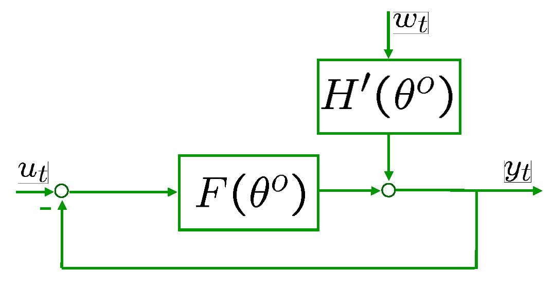
Consider the ARMA system
where ![]() and
and ![]() is an independent sequence of zero mean
Gaussian random variables
with variance 1. 1025 data points were generated.
is an independent sequence of zero mean
Gaussian random variables
with variance 1. 1025 data points were generated.
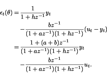
The model ![]() has predictor
and
prediction error given by
has predictor
and
prediction error given by
In order to form a confidence
region for ![]() we calculated
we calculated
and then computed
using the Gordon
group. Next we
discarded those values of ![]() and
and ![]() for which zero was among the 12 largest and smallest values of
for which zero was among the 12 largest and smallest values of ![]() and
and![]() .
.
According to
Theorem 2, ![]() belongs to the
constructed
region with probability at least
belongs to the
constructed
region with probability at least ![]() .
.
The
obtained confidence region is the blank area in Figure 7.
Using the algorithm for the
construction of ![]() , we have
obtained a bounded confidence
set with a guaranteed probability based on a finite number of data
points. As no asymptotic theory is involved, this is a rigorous
finite sample result. For comparison, we have in Figure 7
also plotted the 95% confidence ellipsoid obtained using the
asymptotic theory (e.g. L. Ljung, "System identification - Theory for
the user, Chapter 9, 1999, Prentice Hall). The two confidence regions
are of similar shape and size in this case.
, we have
obtained a bounded confidence
set with a guaranteed probability based on a finite number of data
points. As no asymptotic theory is involved, this is a rigorous
finite sample result. For comparison, we have in Figure 7
also plotted the 95% confidence ellipsoid obtained using the
asymptotic theory (e.g. L. Ljung, "System identification - Theory for
the user, Chapter 9, 1999, Prentice Hall). The two confidence regions
are of similar shape and size in this case.
![\includegraphics[width=7.5cm]{armacolourg12asymp.eps}](equations-figures/img192.png)
Fig.7 Non-asymptotic confidence
region for ![]() (blank
region) and asymptotic confidence
ellipsoid.
(blank
region) and asymptotic confidence
ellipsoid. ![]() = true
parameter,
= true
parameter, ![]() =
estimated parameter
using a prediction error method.
=
estimated parameter
using a prediction error method.
Example 2 - A closed-loop system
This example was
originally introduced in Garatti et al. (2004)
to demonstrate that the
asymptotic theory of PEM can at times deliver misleading results even
with a large number of data points. It is re-examined here to show
how
LSCR works in this challenging situation.
Consider the system of Figure 8
where
 |
|||
![]() is white Gaussian noise with
variance 1 and the reference
is white Gaussian noise with
variance 1 and the reference ![]() is also white Gaussian, with
variance
is also white Gaussian, with
variance![]() . Note that the
variance of the reference signal is
very small as compared to the noise variance, that is there is poor
excitation. The present
situation - though admittedly artificial - is a simplification of what
often happens in practical applications of identification, where poor
excitation is due
to the closed-loop operation of the system.
. Note that the
variance of the reference signal is
very small as compared to the noise variance, that is there is poor
excitation. The present
situation - though admittedly artificial - is a simplification of what
often happens in practical applications of identification, where poor
excitation is due
to the closed-loop operation of the system.
2050 measurements of ![]() and
and ![]() were generated to be used for
identification.
were generated to be used for
identification.
We first use PEM identification.
A full order model was identified.
The amplitude Bode diagrams of the transfer function from ![]() to
to ![]() of
the identified model and of the real system are plotted in
Figure 9. From the plot, a big mismatch between the real
plant and the identified model is apparent, a fact that does not come
too much of a surprise considering that the reference signal is poorly
exciting.
of
the identified model and of the real system are plotted in
Figure 9. From the plot, a big mismatch between the real
plant and the identified model is apparent, a fact that does not come
too much of a surprise considering that the reference signal is poorly
exciting.
An analysis conducted in Garatti et al. (2004)
shows that,
when ![]() , the
asymptotic PEM identification cost has two isolated
global minimizers, one is
, the
asymptotic PEM identification cost has two isolated
global minimizers, one is ![]() and the second
is a spurious
parameter which we denote
and the second
is a spurious
parameter which we denote ![]() . When
. When![]() but small as
is the case
in our actual experiment,
but small as
is the case
in our actual experiment, ![]() does not
minimize the asymptotic
cost anymore, but random fluctuations in the identification cost due to
the finiteness of the data points may as well result in that the
estimate gets trapped near the spurious
does not
minimize the asymptotic
cost anymore, but random fluctuations in the identification cost due to
the finiteness of the data points may as well result in that the
estimate gets trapped near the spurious ![]() , generating a
totally wrong identified model.
, generating a
totally wrong identified model.
![\includegraphics[width=7.5cm]{PEM.eps}](equations-figures/img205.png)
But, let us now see what we
obtained as a 90% confidence region with the asymptotic theory.
Figure 10 displays the confidence region in
the frequency domain: surprisingly, it concentrates around the
identified model, so that in a real identification application where
the
true transfer function is not known we would conclude that the
estimated model is reliable, a totally misleading result.
![\includegraphics[width=7.5cm]{PEM-uncertainty.eps}](equations-figures/img207.png)
Return now to the LSCR approach.
LSCR was used in a totally "blind"
manner, with no concern at
all for the existence of local minima: the method
is guaranteed by theory and it works in all possible situations.
The
prediction error is given by
We used a Gordon
group with 2048
elements, and computed
in the parameter space. We
excluded the regions where 0
was among the 34 smallest or largest values of any of the three
correlations above to obtain a ![]() confidence set (see Theorem 2). The
confidence set is shown in Figure
11.
confidence set (see Theorem 2). The
confidence set is shown in Figure
11.
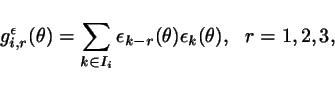
The set consists of two separate regions,
one
around the true parameter ![]() and one around
and one around
![]() . This
illustrates the global features of the
approach: LSCR produces two separate regions as the overall confidence
set because information in the data is intrinsically ineffective in
telling us which one of the two regions contain the true parameter.
. This
illustrates the global features of the
approach: LSCR produces two separate regions as the overall confidence
set because information in the data is intrinsically ineffective in
telling us which one of the two regions contain the true parameter.
Figures 12 and 13 show the
close-ups of the two regions. The ellipsoid in
Figure 12 is the 90% confidence set obtained with the
asymptotic
PEM theory: when the PEM estimate gets trapped near ![]() , the
confidence ellipsoid is centered around this spurious
, the
confidence ellipsoid is centered around this spurious ![]() because the PEM asymptotic theory is local in nature (it is based on a
Taylor expansion) and is therefore unable to explore locations far from
the identified model. This is the reason why in
Figure 10 we obtained a frequency domain
confidence region unable to capture the real model uncertainty. The
reader is referred to Garatti et al. (2004)
for more details.
because the PEM asymptotic theory is local in nature (it is based on a
Taylor expansion) and is therefore unable to explore locations far from
the identified model. This is the reason why in
Figure 10 we obtained a frequency domain
confidence region unable to capture the real model uncertainty. The
reader is referred to Garatti et al. (2004)
for more details.
![\includegraphics[width=7.5cm]{example-closed-LSCR1.eps}](equations-figures/img219.png)
Fig.12 Asymptotic confidence
90% ellipsoid, and the part of the non-asymptotic
confidence set around ![]() .
.
![\includegraphics[width=7.5cm]{example-closed-LSCR2.eps}](equations-figures/img220.png)
LSCR properties
Theorems 1 and 2 quantify the probability
that
belongs to the constructed regions. However, these theorems deal only
with one side of the story. In fact, a good evaluation method must have
two properties:
- the provided region must have guaranteed probability (and this is what Theorems 1 and 2 deliver);
- the region must be bounded, and
concentrate around as the number
of
data points increases.
Securing this second
property requires choosing ![]() and
and ![]() in
a suitable way, and the correct choice depends on the model
class. For a general discussion, particularly in connection with ARMA
and ARMAX models, see Campi and Weyer (2005).
in
a suitable way, and the correct choice depends on the model
class. For a general discussion, particularly in connection with ARMA
and ARMAX models, see Campi and Weyer (2005).
Presence of unmodeled dynamics
LSCR can also be used in the
presence
of unmodeled dynamics.
General ideas
are discussed here by means of two simple examples:
- identifying
a full-order transfer
function between
 and
and  , without
deriving a model for the noise;
, without
deriving a model for the noise;
- presence of unmodeled dynamics in the
to transfer function.
Identification without a noise model: an example
Consider the system
Suppose that the structure of the ![]() to
to ![]() transfer function is known. Instead, the
noise
transfer function is known. Instead, the
noise ![]() describes all other sources of variation in
describes all other sources of variation in ![]() apart from
apart from ![]() and
we do not want to make any assumption on how
and
we do not want to make any assumption on how ![]() is generated.
Correspondingly, we want our results regarding the value of
is generated.
Correspondingly, we want our results regarding the value of ![]() to be valid
with no limitations whatsoever on the deterministic noise sequence
to be valid
with no limitations whatsoever on the deterministic noise sequence ![]() .
.
Assume that we
have access to the system for experimentation: we generate a
finite number, say 7 for the sake of simplicity, of input data and -
based on the collected
outputs - we are asked to construct a confidence interval ![]() for
for ![]() of guaranteed
probability.
of guaranteed
probability.
The problem is challenging: since
the noise can be whatever, it seems that the observed
data are unable to give us a hand in constructing a confidence region.
In fact, for any given ![]() and
and ![]() , a suitable choice of the
noise sequence can lead to any observed output signal! Let us see how
LSCR gets around this problem.
, a suitable choice of the
noise sequence can lead to any observed output signal! Let us see how
LSCR gets around this problem.
Before proceeding, we would like
to clarify what is meant here by "guaranteed probability".
We said that ![]() is regarded as
a deterministic sequence, and the
result is required to hold true for any
is regarded as
a deterministic sequence, and the
result is required to hold true for any ![]() , that is
uniformly in
, that is
uniformly in ![]() . The
stochastic element is instead the input sequence: we will
select
. The
stochastic element is instead the input sequence: we will
select ![]() according to a random generation
mechanism and we require
that
according to a random generation
mechanism and we require
that ![]() with a given
probability, where
the probability is with respect to the random choice of
with a given
probability, where
the probability is with respect to the random choice of ![]() .
.
We first indicate the input design
and
then the procedure for construction of the confidence interval ![]() .
.
Input
design
Let ![]() ,
, ![]() , be
independent and identically distributed with distribution
, be
independent and identically distributed with distribution
Procedure
for construction of
the confidence interval
Rewrite the system as a model with
generic parameter ![]() :
:
Construct a predictor by
dropping the noise term ![]() :
:
Next, we compute the prediction
errors ![]() from the
observed data for
from the
observed data for ![]() and calculate
and calculate
Then, we take different averages of these functions. Precisely, we form
8 averages of the form:
where the sets ![]() are subsets
of
are subsets
of ![]() containing the
elements highlighted by a bullet in
the table below. For instance:
containing the
elements highlighted by a bullet in
the table below. For instance: ![]() ,
, ![]() , etc.
, etc.
The confidence interval is where at
least two functions are below zero and at least two functions are above
zero.
A simulation example was run with ![]() and where the
noise
sequence was as shown in Figure 14. This
noise sequence was obtained as a realization of
a biased independent Gaussian process with mean 0.5 and variance 0.1.
The obtained
and where the
noise
sequence was as shown in Figure 14. This
noise sequence was obtained as a realization of
a biased independent Gaussian process with mean 0.5 and variance 0.1.
The obtained ![]() functions are
given in Figure 15.
functions are
given in Figure 15.
We located the
interval
where at least two functions were below zero and at least two were
above
zero, obtaining the interval in Figure 15. Generalizing the theory
for the case of no unmodelled dynamics,
one can establish that the obtained interval has exacxt probability 0.5
of containing the true ![]() (see Campi and Weyer (2006)).
(see Campi and Weyer (2006)).
![\includegraphics[width=7cm]{noise-noise-free-example.eps}](equations-figures/img283.png)
![\includegraphics[width=7.5cm]{noise-free-correlations.eps}](equations-figures/img284.png)
Fig.15 The
Unmodeled dynamics in the transfer function between
u and y: an example
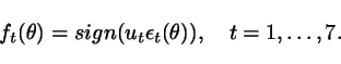
Suppose that a system has structure
while - for estimation purposes -
we use the reduced order model
The noise can be whatever, and we
regard ![]() as a generic
unknown deterministic signal.
as a generic
unknown deterministic signal.
After determining a region for the
parameter ![]() one sensible
question to ask is: does this region
contain with a given probability the system parameter
one sensible
question to ask is: does this region
contain with a given probability the system parameter ![]() linking
linking ![]() to
to ![]() ?
?
Reinterpreting the above question
we are asking whether the projection of the true transfer function ![]() onto the 1-dimensional space spanned
by constant transfer functions is contained in the estimated set with a
certain probability.
onto the 1-dimensional space spanned
by constant transfer functions is contained in the estimated set with a
certain probability.
Input
design
Let ![]() ,
, ![]() , be
independent and identically distributed with distribution
, be
independent and identically distributed with distribution
Procedure
for construction of
the confidence interval
Construct a prediction by
dropping the noise term ![]() whose
characteristics are unknown:
whose
characteristics are unknown:
Next, we compute the prediction
errors ![]() from the
observed data for
from the
observed data for ![]() and calculate:
and calculate:
Then, we take the average of some of
these functions in many
different ways. Precisely, we form 8 averages of the form:
where the sets ![]() are subsets
of
are subsets
of ![]() containing the
elements highlighted by a bullet in
the table below. For instance:
containing the
elements highlighted by a bullet in
the table below. For instance: ![]() ,
, ![]() , etc.
, etc.
The confidence interval
is where at least two functions are below zero and at least two
functions are above zero.
A simulation example was run with ![]() ,
, ![]() and where the
noise was the
realization of a biased Gaussian process shown in Figure
14. As
and where the
noise was the
realization of a biased Gaussian process shown in Figure
14. As ![]() can only take
on the
values -1, 1 and 0, it is possible that two or more of the
can only take
on the
values -1, 1 and 0, it is possible that two or more of the ![]() functions will
take on the same value on an interval.
This tie is broken
by introducing a random ordering. The obtained
functions will
take on the same value on an interval.
This tie is broken
by introducing a random ordering. The obtained ![]() functions and confidence region are shown in Figure 16.
functions and confidence region are shown in Figure 16.
![\includegraphics[width=7.5cm]{sign-correlations.eps}](equations-figures/img298.png)
Fig.16 The
Generalizing the theory, one can
establish that the obtained interval has exacxt probability 0.5
to contain
the true ![]() (see Campi and Weyer (2006)).
(see Campi and Weyer (2006)).
Nonlinear systems
Here we discuss an example. The reader is
referred to Dalai et al. (2007, to appear in Automatica) for more
details.
Consider the following nonlinear
system
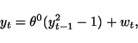
where ![]() is an independent and
symmetrically distributed sequence and
is an independent and
symmetrically distributed sequence and ![]() is an unknown
parameter.
is an unknown
parameter.
This system can be made explicit
with respect to ![]() as follows:
as follows:
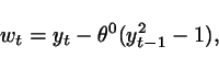
and - by substituting ![]() with a generic
with a generic ![]() and re-naming
the so-obtained right-hand-side
as
and re-naming
the so-obtained right-hand-side
as ![]() - we have
- we have
Second order statistics are in
general not enough to identify the true parameter value for nonlinear
systems. The good news is
that LSCR
can be extended to higher-order statistics with little effort. A
general presentation of the results can be found in Dalai et
al. (2007, to appear in
Automatica). Here, it
suffices to say that we can e.g. consider the
third-order statistic ![]() and the theory
goes through.
and the theory
goes through.
As an example, we generated 9
samples of ![]() ,
, ![]() where
where ![]() were zero-mean Gaussian with
variance 1. Then, we
constructed
were zero-mean Gaussian with
variance 1. Then, we
constructed
where the sets ![]() are subsets
of
are subsets
of ![]() containing the
elements highlighted by a bullet in
the table below. For instance:
containing the
elements highlighted by a bullet in
the table below. For instance: ![]() ,
, ![]() , etc.
, etc.
These
functions are
displayed in Figure 17. The interval marked in
blue is where at least two functions were below zero and at least two
were above zero and has exact probability 0.5 of containing ![]() .
.
![\includegraphics[width=7.5cm]{nonlinear-correlations.eps}](equations-figures/img318.png)
Closed-loop
Closed-loop systems can be treated within to the open-loop framework by regarding
Gordon's construction of the incident matrix of a group
Given ![]() , the
incident matrix for a group
, the
incident matrix for a group ![]() of subsets of
of subsets of ![]() is a matrix
whose
is a matrix
whose ![]() element is
element is ![]() if
if ![]() and zero
otherwise. In L. Gordon,
"Completely separating groups in subsampling", Annals of Statistics,
vol.2, pp.572-578, the following
construction procedure for an incident
matrix
and zero
otherwise. In L. Gordon,
"Completely separating groups in subsampling", Annals of Statistics,
vol.2, pp.572-578, the following
construction procedure for an incident
matrix ![]() is proposed
where
is proposed
where ![]() and
the group has
and
the group has ![]() elements.
elements.
Let ![]() , and
recursively
compute (
, and
recursively
compute (![]() )
)
![\begin{displaymath}
R(2^k-1)=\left[ \begin{array}{ccc} R(2^{k-1}-1) & R(2^{k-1}-...
...}-1) & J-R(2^{k-1}-1) &e \\
0^T & e^T & 1
\end{array}\right],
\end{displaymath}](equations-figures/img347.png)
where ![]() and
and ![]() are,
respectively, a matrix and a vector of all ones, and 0 is a vector of
all zeros. Then, let
are,
respectively, a matrix and a vector of all ones, and 0 is a vector of
all zeros. Then, let
![\begin{displaymath}
\bar{R}=\left[ \begin{array}{c} R(2^l-1) \\
0^T
\end{array}\right].
\end{displaymath}](equations-figures/img350.png)
Gordon (1974) also gives
construction of groups when the number of data points is different from
![]() .
.
Papers
M.C. Campi and E. Weyer.Guaranteed non-asymptotic confidence regions in system identification.
Automatica, 41:1751-1764, 2005.
(the downloadable file is an extended version (with all proofs) of the Automatica paper)
M.C. Campi and E. Weyer.
Identification with finitely many data points: the LSCR approach.
Semi-plenary presentation. In Proc. Symposium on System Identification, SYSID 2006, Newcastle, Australia, 2006.
M. Dalai, E. Weyer and M.C. Campi.
Parameter Identification for Nonlinear Systems: Guaranteed Confidence regions through LSCR.
Automatica, 43:1418-1425, 2007.
Other related papers are downloadable from M.C. Campi's webpage